Exponential Fitting, Separable Least Squares, and Quahogs - Cleve Moler on Mathematics and Computing

[poster]

We have been investigating a recent bug report about fitnlm, the Statistics and Machine Learning Toolbox function for robust fitting of nonlinear models.

Contents

• Quahogs
• Acidification
• Separable Least Squares
• Centering Data
• Exponential Fitting
• Results
• Software
• Thanks

Quahogs



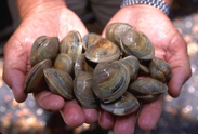The bug report comes from Greg Pelletier, an independent research scientist and biogeochemical modeler in Olympia, Washington. Greg has been studying the vulnerability of sensitive marine organisms to increases in ocean acidification. One of the most important of these organisms is Mercenaria mercenaria, the hard clam.

Especially here in New England, hard clams are known by their traditional Native American name, quahog. They have a well-deserved reputation for making excellent clam chowder.

Acidification

We are all aware of increasing levels of carbon dioxide in the earth's atmosphere. We may not be as aware of the effect this increase has on the health of the earth's oceans. According to NOAA, the ocean absorbs about 30% of the atmospheric carbon dioxide.

A definitive and controversial 2009 paper by Justin Ries and colleagues, then at the Woods Hole Oceanographic Institution, is "Marine calcifiers exhibit mixed responses to CO2-induced ocean acidification", https://doi.org/10.1130/G30210A.1. The hard clam example in Greg's bug report comes from figure 1K in the Ries et al. paper.

The independent variable in experiments is the ratio of alkalinity of sea water to the concentration of dissolved inorganic carbon. The dependent variable is the calcification rate, which compares how fast the organism builds its shells to how fast the shells are dissolving.



Separable Least Squares

The model chosen by Ries at al. is

$$ y \approx \beta_1 + \beta_2 e^{\lambda t} $$

where $t$ is the ratio of alkalinity to dissolved carbon and $y$ is the calcification rate. The data have only four distinct values of $t$, with several observations of $y$ at each value.

The parameters $\beta_1$, $\beta_2$ and $\lambda$ are determined by least squares curve fit. This is a separable least squares problem. For any given value of $\lambda$, the parameters $\beta_1$ and $\beta_2$ occur linearly and the least squares solution can be obtained by MATLAB's backslash.

Gene Golub and Victor Pereyra described separable least squares in 1973 and proposed solving it by a variable projection algorithm. Since 1973 a number of people, including Pereyra, Linda Kaufman, Fred Krogh, John Bolstadt and David Gay, have contributed to the development of a series of Fortran programs named varpro. In 2011, Dianne O'Leary and Burt Rust created a MATLAB version of varpro. Their report, https://www.cs.umd.edu/~oleary/software/varpro/, is a good background source, as well as documentation for varpro.m.

I have a section on separable least squares, and an example, expfitdemo, in NCM, Numerical Computing with MATLAB. I have modified expfitdemo to work on Greg's quahogs problem.

Centering Data

It turns out that the problem Greg encountered can be traced to the fact that the data are not centered. The given values of $t$ are all positive. This causes fitnlm to print a warning message and attempt to rectify the situation by changing the degrees of freedom from 22 to 23, but this only makes the situation worse. (We should take another look at the portion of fitnlm that adjusts the degrees of freedom.)

It is always a good idea in curve fitting to center the data with something like

t = t - mean(t)The values of $y$ are already pretty well centered. Rescaling $y$ with

y = 10000*ymakes interpretation of results easier.

Exponential Fitting

With the data centered and scaled, we have three different ways of tackling Greg's problem. All three methods agree on the results they compute.

• fitnlm. Treats all parameters as if they were nonlinear. Computes statistical quantities such as R-squared and RMS Error.

• varpro. Venerable software history. Only one nonlinear parameter for the quahogs problem. Delivers additional statistical quantities in Regression structure.

• quahogsfit. Textbook separable least squares code. Modification for the quahogs problem of expfitdemo from NCM. Only one nonlinear parameter. No statistics.

Results

• fitnlm

Nonlinear regression model: y ~ param1 + param2*exp(param3*xval)Estimated Coefficients: Estimate SE tStat pValue ________ _______ _______ __________ param1 0.69536 0.1657 4.1964 0.00037344 param2 -0.26482 0.19909 -1.3302 0.19709 param3 -22.218 8.1494 -2.7263 0.012327Number of observations: 25, Error degrees of freedom: 22Root Mean Squared Error: 0.307R-Squared: 0.828, Adjusted R-Squared 0.813F-statistic vs. constant model: 53, p-value = 3.86e-09

• varpro

Linear Parameters: 0.695367 -0.264837Nonlinear Parameters: -22.217495Norm of weighted residual = 1.438935Norm of data vector = 3.545820Expected error of observations = 0.306782Coefficient of determination = 0.828145Regression.t_ratio 4.1962 -1.3301 -2.7264Regression.std_param 0.1657 0.1991 8.1490

• quahogsfit

lambda = -22.2180condX = 4.3882beta = 0.6954 -0.2648normres = 1.4389quahogsfit produces this plot, which can be compared with figure 1K from Ries et al, reproduced above.



Software

The codes for this post are available here quahogs_driver.m and here varpro.m.

Thanks

Thanks to Greg Pelletier for the bug report and to Tom Lane for his statistical expertise.

Get the MATLAB code (requires JavaScript)

Published with MATLAB® R2023a