Speeding-up builtin Matlab functions – part 3 - undocumentedmatlab

[poster]

A recurring theme in this website is that despite a common misperception, builtin Matlab functions are typically coded for maximal accuracy and correctness, but not necessarily best run-time performance. Despite this, we can often identify and fix the hotspots in these functions and use a modified faster variant in our code. I have shown multiple examples for this in various posts (example1, example2, many others).

Today I will show another example, this time speeding up the mvksdensity (multi-variate kernel probability density estimate) function, part of the Statistics toolbox since R2016a. You will need Matlab R2016a or newer with the Stats Toolbox to recreate my results, but the general methodology and conclusions hold well for numerous other builtin Matlab functions that may be slowing down your Matlab program. In my specific problem, this function was used to compute the probability density-function (PDF) over a 1024×1024 data mesh.

The builtin mvksdensity function took 76 seconds to run on my machine; I got this down to 13 seconds, a 6x speedup, without compromising accuracy. Here’s how I did this:

Preparing the work files

While we could in theory modify Matlab’s installed m-files if we have administrator privileges, doing this is not a good idea for several reasons. Instead, we should copy and rename the relevant internal files to our work folder, and only modify our local copies.

To see where the builtin files are located, we can use the which function:

>> which('mvksdensity')C:\Program Files\Matlab\R2020a\toolbox\stats\stats\mvksdensity.mIn our case, we copy \toolbox\stats\stats\mvksdensity.m as mvksdensity_.m to our work folder, replace the function name at the top of the file from mvksdensity to mvksdensity_, and modify our code to call mvksdensity_ rather than mvksdensity.

If we run our code, we get an error telling us that Matlab can’t find the statkscompute function (in line #107 of our mvksdensity_.m). So we find statkscompute.m in the \toolbox\stats\stats\private\ folder, copy it as statkscompute_.m to our work folder, rename its function name (at the top of the file) to statkscompute_, and modify our mvksdensity_.m to call statkscompute_ rather than statkscompute:

[fout,xout,u] = statkscompute_(ftype,xi,xispecified,npoints,u,L,U,weight,cutoff,...We now repeat the process over and over, until we have all copied all the necessary internal files for the program to run. In our case, it tuns out that in addition to mvksdensity.m and statkscompute.m, we also need to copy statkskernelinfo.m.

Finally, we check that the numeric results using the copied files are exactly the same as from the builtin method, just to be on the safe side that we have not left out some forgotten internal file.

Now that we have copied these 3 files, in practice all our attentions will be focused on the dokernel sub-function inside statkscompute_.m, since the profiling report (below) indicates that this is where all of the run-time is spent.

Identifying the hotspots

Now we run the code through the Matlab Profiler, using the “Run and Time” button in the Matlab Editor, or profile on/report in the Matlab console (Command Window). The results show that 99.8% of mvksdensity‘s time was spent in the internal dokernel function, 75% of which was spent in self-time (meaning code lines within dokernel):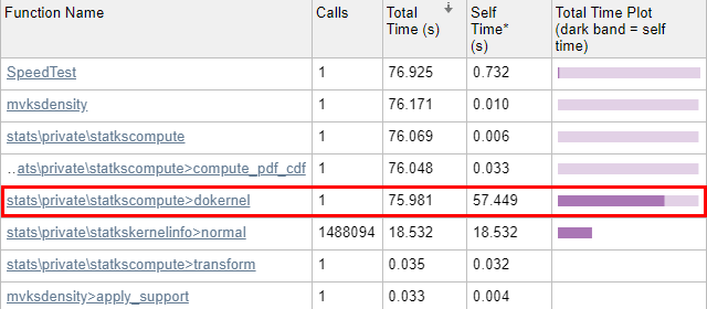
Initial profiling results - pretty slow...

Let’s drill into dokernel and see where the problems are: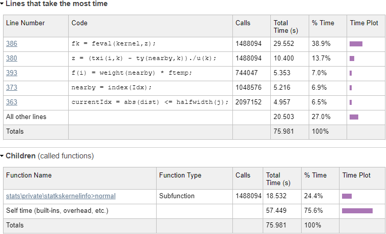
Initial dokernel profiling results

Evaluating the normal kernel distribution

We can immediately see from the profiling results that a single line (#386) in statkscompute_.m is responsible for nearly 40% of the total run-time:

fk = feval(kernel,z);In this case, kernel is a function handle to the normal-distribution function in \stats\private\statkskernelinfo>normal, which is evaluated 1,488,094 times. Using feval incurs an overhead, as can be seen by the difference in run-times: line #386 takes 29.55 secs, whereas the normal function evaluations only take 18.53 secs. In fact, if you drill into the normal function in the profiling report, you’ll see that the actual code line that computes the normal distribution only takes 8-9 seconds – all the rest (~20 secs, or ~30% of the total) is totally redundant function-call overhead. Let’s try to remove this overhead by calling the kernel function directly:

fk = kernel(z);Now that we have a local copy of statkscompute_.m, we can safely modify the dokernel sub-function, specifically line #386 as explained above. It turns out that just bypassing the feval call and using the function-handle directly does not improve the run-time (decrease the function-call overhead) significantly, at least on recent Matlab releases (it has a greater effect on old Matlab releases, but that’s a side-issue).

We now recognize that the program only evaluates the normal-distribution kernel, which is the default kernel. So let’s handle this special case by inlining the kernel’s one-line code (from statkskernelinfo_.m) directly (note how we move the condition outside of the loop, so that it doesn’t get recomputed 1 million times):

...isKernelNormal = strcmp(char(kernel),'normal'); % line #357 for i = 1:m Idx = true(n,1); cdfIdx = true(n,1); cdfIdx_allBelow = true(n,1); for j = 1:d dist = txi(i,j) - ty(:,j); currentIdx = abs(dist) = -halfwidth(j); cdfIdx = currentCdfIdx & cdfIdx; %cdf boundary1, equal or below the query point in all dimension currentCdfIdx_below = dist - halfwidth(j) > 0; cdfIdx_allBelow = currentCdfIdx_below & cdfIdx_allBelow; %cdf boundary2, below the pdf lower boundary in all dimension end end if ~iscdf nearby = index(Idx); else nearby = index((Idx|cdfIdx)&(~cdfIdx_allBelow)); end if ~isempty(nearby) ftemp = ones(length(nearby),1); for k =1:d z = (txi(i,k) - ty(nearby,k))./u(k); if reflectionPDF zleft = (txi(i,k) + ty(nearby,k)-2*L(k))./u(k); zright = (txi(i,k) + ty(nearby,k)-2*U(k))./u(k); fk = kernel(z) + kernel(zleft) + kernel(zright); % old: =feval()+... elseif isKernelNormal fk = exp(-0.5 * (z.*z)) ./ sqrt(2*pi); else fk = kernel(z); %old: =feval(kernel,z); end if needUntransform(k) fk = untransform_f(fk,L(k),U(k),xi(i,k)); end ftemp = ftemp.*fk; end f(i) = weight(nearby) * ftemp; end if iscdf && any(cdfIdx_allBelow) f(i) = f(i) + sum(weight(cdfIdx_allBelow)); endend...This reduced the kernel evaluation run-time from ~30 secs down to 8-9 secs. Not only did we remove the direct function-call overhead, but also the overheads associated with calling a sub-function in a different m-file. The total run-time is now down to 45-55 seconds (expect some fluctuations from run to run). Not a bad start.

Main loop – bottom part

Now let’s take a fresh look at the profiling report, and focus separately on the bottom and top parts of the main loop, which you can see above. We start with the bottom part, since we already messed with it in our fix to the kernel evaluation: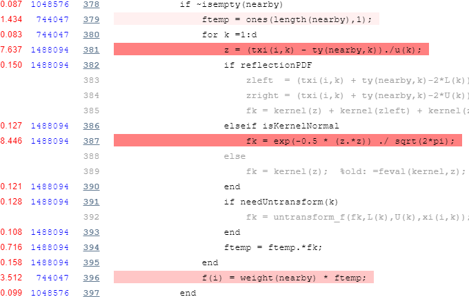

Profiling results for bottom part of the main loop

The first thing we note is that there’s an inner loop that runs d=2 times (d is set in line #127 of mvksdensity_.m – it is the input mesh’s dimensionality, and also the number of columns in the txi data matrix). We can easily vectorize this inner loop, but we take care to do this only for the special case of d==2 and when some other special conditions occur.

In addition, we hoist outside of the main loop anything that we can (such as the constant exponential power, and the weight multiplication when it is constant [which is typical]), so that they are only computed once instead of 1 million times:

...isKernelNormal = strcmp(char(kernel),'normal');anyNeedTransform = any(needUntransform);uniqueWeights = unique(weight);isSingleWeight = ~iscdf && numel(uniqueWeights)==1;isSpecialCase1 = isKernelNormal && ~reflectionPDF && ~anyNeedTransform && d==2;expFactor = -0.5 ./ (u.*u)';TWO_PI = 2*pi;for i = 1:m ... if ~isempty(nearby) if isSpecialCase1 z = txi(i,:) - ty(nearby,:); ftemp = exp((z.*z) * expFactor); else ftemp = 1; % no need for the slow ones() for k = 1:d z = (txi(i,k) - ty(nearby,k)) ./ u(k); if reflectionPDF zleft = (txi(i,k) + ty(nearby,k)-2*L(k)) ./ u(k); zright = (txi(i,k) + ty(nearby,k)-2*U(k)) ./ u(k); fk = kernel(z) + kernel(zleft) + kernel(zright); % old: =feval()+... elseif isKernelNormal fk = exp(-0.5 * (z.*z)) ./ sqrt(TWO_PI); else fk = kernel(z); % old: =feval(kernel,z) end if needUntransform(k) fk = untransform_f(fk,L(k),U(k),xi(i,k)); end ftemp = ftemp.*fk; end ftemp = ftemp * TWO_PI; end if isSingleWeight f(i) = sum(ftemp); else f(i) = weight(nearby) * ftemp; end end if iscdf && any(cdfIdx_allBelow) f(i) = f(i) + sum(weight(cdfIdx_allBelow)); endendif isSingleWeight f = f * uniqueWeights;endif isKernelNormal && ~reflectionPDF f = f ./ TWO_PI;end...This brings the run-time down to 31-32 secs. Not bad at all, but we can still do much better:

Main loop – top part

Now let’s take a look at the profiling report’s top part 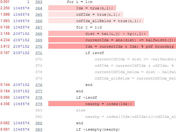of the main loop:

Profiling results for top part of the main loop

Again we note is that there’s an inner loop that runs d=2 times, which we can again easily vectorize. In addition, we note the unnecessary repeated initializations of the true(n,1) vector, which can easily be hoisted outside the loop:

...TRUE_N = true(n,1);isSpecialCase2 = ~iscdf && d==2;for i = 1:m if isSpecialCase2 dist = txi(i,:) - ty; currentIdx = abs(dist) 0; cdfIdx_allBelow = currentCdfIdx_below & cdfIdx_allBelow; %cdf boundary2, below the pdf lower boundary in all dimension end end if ~iscdf nearby = index(Idx); else nearby = index((Idx|cdfIdx)&(~cdfIdx_allBelow)); end end if ~isempty(nearby) ...This brings the run-time down to 24 seconds.

We next note that instead of using numeric indexes to compute the nearby vector, we could use faster logical indexes:

...%index = (1:n)'; % this is no longer neededTRUE_N = true(n,1);isSpecialCase2 = ~iscdf && d==2;for i = 1:m if isSpecialCase2 dist = txi(i,:) - ty; currentIdx = abs(dist) 0; cdfIdx_allBelow = currentCdfIdx_below & cdfIdx_allBelow; %cdf boundary2, below the pdf lower boundary in all dimension end end if ~iscdf nearby = Idx; % not index(Idx) else nearby = (Idx|cdfIdx) & ~cdfIdx_allBelow; % no index() end end if any(nearby) ...This brings the run-time down to 20 seconds.

We now note that the main loop runs m=1,048,576 (=1024×1024) times over all rows of txi. This is expected, since the loop runs over all the elements of a 1024×1024 mesh grid, which are reshaped as a 1,048,576-element column array at some earlier point in the processing, resulting in a m-by-d matrix (1,048,576-by-2 in our specific case). This information helps us, because we know that there are only 1024 unique values in each of the two columns of txi. Therefore, instead of computing the “closeness” metric (which leads to the nearby vector) for all 1,048,576 x 2 values of txi, we calculate separate vectors for each of the 1024 unique values in each of its 2 columns, and then merge the results inside the loop:

...isSpecialCase2 = ~iscdf && d==2;if isSpecialCase2 [unique1Vals, ~, unique1Idx] = unique(txi(:,1)); [unique2Vals, ~, unique2Idx] = unique(txi(:,2)); dist1 = unique1Vals' - ty(:,1); dist2 = unique2Vals' - ty(:,2); currentIdx1 = abs(dist1)